Chapter 1 Application Project:

The emergence of the SARS-CoV-2 virus in late 2019 and its subsequent rapid global spread changed the world as we know it. The World Health Organization declared the spread to be a pandemic, known as COVID-19, in March 2020, recommending precautions such as cleanliness, social distancing, and the use of face masks. Mathematics in general, and functions in particular, provide us with the tools to build models that help us understand the spread of contagious diseases and the nature of epidemics or pandemics. This project will provide an introduction to the way such models can be built. Good mathematical models can not only help us understand how an epidemic or pandemic runs its course, but can also be used in decision making regarding mitigation measures and allocation of resources in order to save lives!

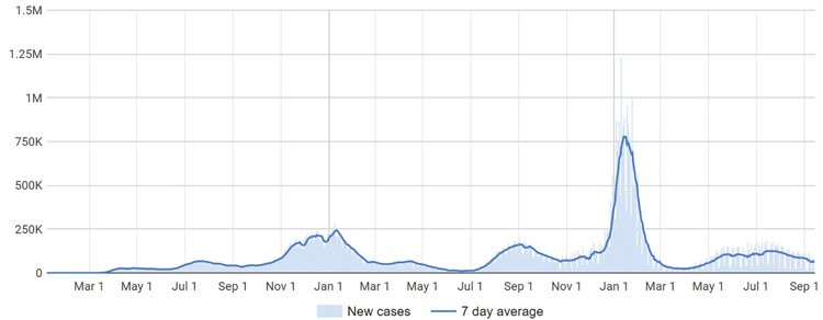
A combination of bar and line graph where the bars represent the number of new cases and the line represents the 7-day average. The x-axis represents months spanning from January 1, 2020 to September 1, 2022. The y-axis represents number of infections spanning from 0 to 1.5 million. The distribution of infections matches the curve of the 7-day average with most of the data staying below 125,000 infections. Between November 1, 2020 and February 1, 2021, the number of infections rises to 250,000 before falling back down. Between December 1, 2022 and March 1, 2022, the number of average infections peaks just over 750,000 while the new cases peaks 1.25 million before falling back down.

Source: Google COVID-19 Open Data (goo.gle/COVID-19-open-data)

COVID-19 was of particular concern early on when there were no vaccines available and the overwhelming majority of the population had not yet been exposed to the virus, making them susceptible to it. In this project, we will build a rudimentary mathematical model to describe and understand the spread of the disease on a college campus of $\mathrm{25,000}$ students, with the following simplifying assumptions.

• Anyone catching the disease eventually recovers.

• After recovery, any affected individual becomes immune (i.e., we will assume there are no reinfections).

• There are no vaccines yet available.

Further, we will partition the campus population into the following three subsets:

• Infected, meaning those students carrying the virus (with or without symptoms)

• Recovered, meaning those students who cannot be reinfected (due to our simplifying assumptions)

• Susceptible, meaning those who have not yet had the virus and can still potentially get it

Note that the sizes of these sets depend on time—that is, they are functions of time—while at any moment in time, they always add up to the total of $\mathrm{25,000}$ students. We will denote these subsets of people by $P_i$, $P_r$, and $P_s$, respectively.

1. Figure 2 illustrates how the size of the infected subpopulation $P_i$ may depend on time t.

   

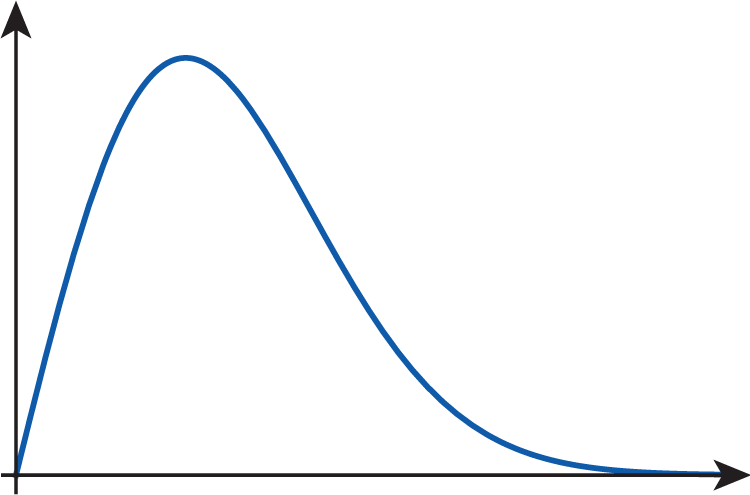
   The first quadrant of a cartesian graph with an unlabeled curve. The curve starts at the origin and rises quickly and begins descending similarly but the descent slows as it continues.

   1. What are the independent and dependent variables of this function?

   2. Use the features of the graph to explain why it seems realistic. What does it tell you about the way the infection runs its course on campus?

   3. Use function notation to write an equation expressing the fact that the numbers of infected, recovered, and susceptible student populations sum up to $\mathrm{25,000}$ at any given time. (Hint: remember that $P_i$, $P_r$, and $P_s$ are functions of time t.)

2. How would you expect the number of susceptible students to change over time? Explain and sketch a possible graph of the size of $P_s$ over time.

3. Answer Question 2 and sketch a possible graph for the recovered subpopulation $P_r$.

Throughout the COVID-19 pandemic, the daily reports included (among other data) the number of new cases on a given day. Note that this is an important measure of how fast the infection spreads. In other words, using the general concept of "rate" being "change divided by time," you can think of that number as the rate of increase in size of the set of people who have caught the disease. (You will learn more about rates starting in Chapter 2.) Throughout the next few questions, we are going to build an equation modeling the progression of the disease in the college population. Our assumptions will be as follows. New infections are always the result of interactions between members of the infected and susceptible populations. Even though not all interactions result in new infections, a certain percentage of them do (note that this percentage can be decreased by mitigation measures, such as masking or distancing). We will assume that the number of interactions is directly proportional to both $P_s$ and $P_i$.

4. Find a formula for $N\left(t\right)$, the number of daily new infections, given the assumptions above. (The constant of proportionality in this case is called the transmission coefficient. Let us denote it by b.)

5. Given that, on average, an infected person is contagious for about ten days, explain why we can expect approximately ${\displaystyle \frac{P_i\left(t\right)}{10}}$ students to recover daily. Discuss the limitations of this model.

6. 1. Given that some students get infected while others recover every single day, use your answers to Questions 4 and 5 to find a formula for $\widehat{P_i}\left(t\right)$, the daily increase in numbers of the infected student population.

   2. Use your formula to predict the number of new infections on a day when $500$ students are carrying the virus and $1000$ have already recovered. Use the value $b=0.000025$ for the transmission coefficient.

7. Use the equation obtained in Question 6 to predict the size of the susceptible population (i.e., those who have not caught the virus) when the epidemic peaks on campus. (Hint: Find what value of $P_s$ predicts a zero daily increase in $P_i$ for the first time. Round to the nearest integer. Then check that the following day, the predicted daily increase in $P_i$ is negative.)