Chapter 7 Application Project:

Speeding Up to Slow Down

Though often overlooked by nonenthusiasts, one of the most important characteristics of a car's engine is the torque it generates, and subsequently, its distribution across the rpm range. A graph of the torque an engine produces, as a function of rpm, is referred to as the engine's torque curve. In this project, we will investigate the effect of the torque curve on a car's power, especially on its performance in stop-and-go city driving.

In physics texts, torque is introduced as the measure of a force's ability to rotate an object about an axis. Specifically, when a force is rotating a mass or a rigid body around an axis, its torque equals the product of the force and the perpendicular distance of its line of action from the axis of rotation. (We will give a precise definition in Section 11.4.) In automotive technology, torque is the measure of the engine's ability to rotate the driveshaft, and ultimately, the drive wheels. It is responsible for a car's acceleration and, simply put, torque is what you feel when stepping on the accelerator pedal.

As you would expect, the engine's torque rating is strongly connected to the car's power, which is measured in horsepower (hp) or kilowatts (kW). We will first explore this relationship, then examine how the shape of the torque curve influences acceleration and driving feel, and later we will use integration to calculate the total energy required to accelerate a car.

In general, power is defined as the instantaneous rate at which work is done, given by the following formula.

$P={\displaystyle \frac{\mathit{d}W}{\mathit{d}t}}$    (1)

Since we can think of work as the transfer of energy (usually denoted by E), an alternative equation for power is as follows.

$P={\displaystyle \frac{\mathit{d}E}{\mathit{d}t}}$    (1a)

Though we will not derive it here, the (instantaneous) power of an automotive engine with a torque output of τ is given by the following equation.

$P=\tau \cdot \omega$    (2)

The value of ω is the angular velocity of the driveshaft, calculated as follows, where θ is the angle of rotation of the driveshaft in radians.

$\omega ={\displaystyle \frac{\mathit{d}\theta }{\mathit{d}t}}$

1. If $P\left(t\right)$ denotes the power output of an engine as a function of time, use Equation (1) above to show that the total work done by the engine in accelerating the car from $t=t_0$ to $t=t_1$ can be obtained from the subsequent formula.

   $W={\displaystyle {\int }_{t_0}^{t_1}P\left(t\right)\mathit{d}t}$

2. 1. Given that angular velocity is measured in radians per second, and that rpm expresses the number of full revolutions per minute, find the conversion factor between angular velocity and rpm. In other words, what angular velocity (in $\mathrm{rad}/\sec$) corresponds to 1 rpm?

   2. Suppose an engine's torque output is ${\rm T}\mathrm{lb-ft}$. when the engine speed is N rpm. Use Equation (2) and your answer to part a. to express the engine's power P in $\mathrm{lb-ft}/\sec$ at that instant.

   3. Given that $1\text{horsepower}$ (hp) equals $500{\displaystyle \frac{\mathrm{lb-ft}}{\mathrm{s}}}$, use your answer to part b. to verify the given formula.

      $\text{power}={\displaystyle \frac{\text{torque}\times \text{rpm}}{5252}}$

      Power in the above formula is measured in hp, while torque is measured in $\mathrm{lb-ft}$. However, in general, power is most often expressed using the metric system, in watts (W) or kilowatts (kW). One watt of power performs one joule of work in one second, demonstrated as follows.

      $1\mathrm{W}=1{\displaystyle \frac{\mathrm{J}}{\mathrm{s}}}=1\mathrm{kg}\cdot {\displaystyle \frac{{\mathrm{m}}^2}{{\mathrm{s}}^3}}$

      When referring to automotive power, we note that since $1\text{watt}$ approximately equals ${\displaystyle \frac{1}{746}\text{horsepower}}$, we obtain the following conversions between units.

      $1\mathrm{hp}=746\mathrm{W}=0.746\mathrm{kW}$

3. Suppose the graphs in Figure 1 show the torque and power curves of the 2015 and 2021 Brand X car models, respectively. Examine the curves and answer the questions below.

   

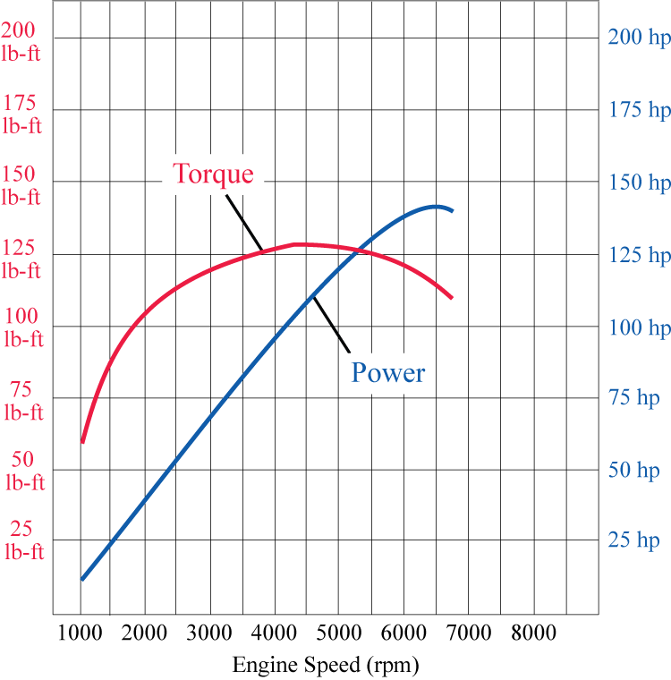
   A graph depicting the torque and power of the 2015 model car of brand X. The x-axis is labeled as Engine Speed (rpm) from 500 to 9000 by 500. The y-axis has two separate labels. The first label is associated with torque and is labeled from 0 pound-feet to 200 pound-feet by 25. The second label is associated with power and is labeled from 0 horsepower to 200 horsepower by 25. The graph for Torque starts at approximately (1000, 60), curves upward to peak at approximately (4500, 127), then curves downward to end at approximately (6750, 112). The graph for Power starts at approximately (1000, 12) and increases linearly until approximately (5500, 130) when its growth slows and begins curving, peaking at approximately (6500, 140) and curves downward to end at approximately (6750, 137).

   

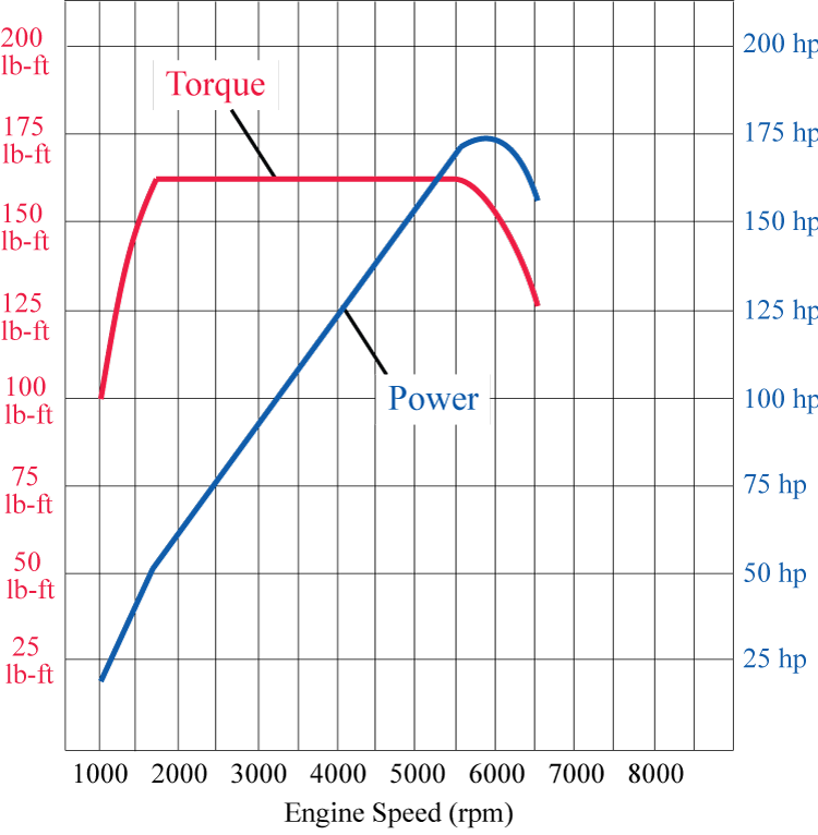
   A graph depicting the torque and power of the 2021 model car of brand X using the same labels as the previous graph. The graph for Torque starts at (1000, 100) and rises sharply to approximately (1750, 162), remains constant to approximately (5500, 162), and curves gradually down ending at (6500, 127). The graph for Power starts at approximately (1000, 20), rises linearly to approximately (1700, 50), rises linearly at a different rate to approximately (5500, 170), then curves downward to end at approximately (5500, 155).

   1. Notice that in both graphs of Figure 1, the power curve intersects the torque curve at $5252\mathrm{rpm}$. Is that a coincidence? Explain.

   2. Use Figure 1a as well as the formula you obtained in Question 2c to estimate the horsepower range generated by the 2015 car's engine when the engine is revved from $2000$ to $3500\mathrm{rpm}$. (Answers will be approximate. Note that this is a typical rpm range in city traffic. Also notice how different your answer is from the "peak horsepower" rating typically advertised for consumers!)

   3. Repeat part b. for the 2021 edition of the car.

   4. From your answers above, which car would you expect to have better acceleration in typical city driving conditions?

   5. Summarize your findings in this problem by explaining why having a "flat" torque curve (as in the second illustration above) is advantageous in city driving. (This is typical with certain turbocharged or large displacement engines.)

4. Suppose a certain car's torque curve can be approximated by the function

   ${\rm T}\left(x\right)=200\sin {\displaystyle \frac{x}{3000}}$

   on the interval $\left(0,6500\right)$, where the independent variable x stands for rpm.

   1. Find a formula for the power function $P\left(x\right)$ (i.e., the horsepower as a function of engine speed) on the same interval.

   2. Use a graphing utility to graph the functions $T\left(x\right)$ and $P\left(x\right)$ on the interval $\left(500,6500\right)$.

   3. Suppose we accelerate the car (without shifting gears) from $0$ to $4000$ rpm in $4$ seconds. Assuming that the rate of change of the engine speed is constant, use your answer from part a. to express the engine's output in hp as a function of time (in seconds) during the acceleration (i.e., find the formula for $P\left(t\right)$).

   4. Convert your answer in part c. to kilowatts to obtain a formula for the engine's output in kilowatts as a function of time. Then use integration by parts to find the total work done by the engine, in kilojoules, during this acceleration run. (Hint: Use the formula from Question 1.)

5. 1. Suppose we accelerate the 2015 Brand X car model from $1000\mathrm{rpm}$ to $3500\mathrm{rpm}$ in $5$ seconds, without changing gears and while keeping the rate of change of engine speed constant. Use the Trapezoidal Rule and Figure 1a to estimate the work done by the engine. Express your answer in kilojoules. (Answers will be approximate.)

   2. Repeat part a. above for the 2021 Brand X car model, using Figure 1b.

   3. Explain why car performance enthusiasts and tuners often refer to torque or power curves by exclaiming, "I want as much area under the curve as possible."

   4. From your answers above, as well as those given to Question 3, would you prefer a "flat" or a "peaky" torque curve for city driving? Why? (There are no right or wrong answers.)

6. Figure 2 shows the torque and performance curves of various Tesla models.

   

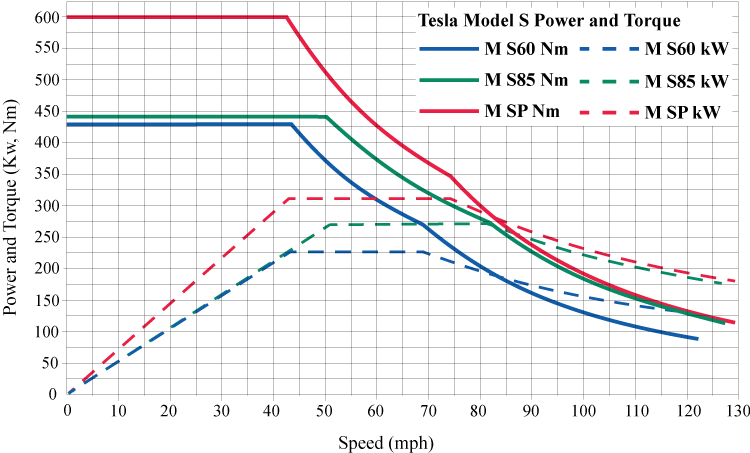
   A graph of the power and torque of three Tesla car models, S60, S85, and SP. The x-axis is labeled Speed (mph), from 0 to 130 by 5. The y-axis is labeled Power and Torque (Kw, Nm), from 0 to 600 by 25.

   Tesla Model S60: The graph for torque starts at approximately (0, 425) and is constant until approximately (44, 425), curves gradually downward to approximately (68, 275), creating a slight cusp as it curves gradually downward further to end at approximately (122, 90). The graph for power starts at (0, 0) and rises linearly to approximately (43, 225), stays constant to approximately (68, 225), and curves gradually downward ending at approximately (122, 125).

   Tesla Model S85: The graph for torque starts at approximately (0, 440) and is constant until approximately (50, 440), curves gradually downward to approximately (82, 275), creating a slight cusp as it curves gradually downward further to end at approximately (127, 112). The graph for power starts at (0, 0) and rises linearly to approximately (51, 270), stays constant to approximately (82, 270), and curves gradually downward ending at approximately (127, 175).

   Tesla Model SP: The graph for torque starts at approximately (0, 600) and is constant until approximately (43, 600), curves gradually downward to approximately (74, 350), creating a slight cusp as it curves gradually downward further to end at approximately (129, 112). The graph for power starts at (0, 0) and rises linearly to approximately (43, 312), stays constant to approximately (74, 225), and curves gradually downward ending at approximately (129, 177).

   Source: Dr. Grzegorz Sieklucki, "An Investigation into the Induction Motor of Tesla Model S Vehicle"

   1. By visually examining the Tesla torque curves, explain the fundamental difference between them and those we discussed above.

   2. Based upon your observations about the graphs, explain why most electric cars have impressive acceleration in stop-and-go city traffic.