Chapter 9 Conceptual Project:

Curve Control

In this project, you will be introduced to a class of parametric curves called Bézier curves. They are important for their applications in engineering, computer graphics, and animation. This class of curves is named after Pierre Bézier (1910–1999), a design engineer for the French automaker Renault, who first demonstrated these curves’ use in designing automobile bodies in the 1960s. The design advantage of Bézier curves lies in the fact that they can easily be manipulated by moving around their so-called control points. In addition, it is easy to smoothly join together several Bézier curves for more complicated shapes.

1. The linear Bézier curve $B_{0,1}\left(t\right)$ from $P_0\left(a_0,b_0\right)$ to $P_1\left(a_1,b_1\right)$ is simply the line segment connecting the two points (note that $P_0$ and $P_1$ are the only control points in this case). Verify that this curve can be parametrized as

   $B_{0,1}\left(t\right)=\left(1-t\right)P_0+t{P}_1$, $t\in \left[0,1\right]$.

   and find $x\left(t\right)$ and $y\left(t\right)$ corresponding to this parametrization. (In this and subsequent questions, control points will be labeled $P_1\left(a_1,b_1\right)$, $0\le i\le 3$.)

2. The Bézier curve $B_{0,1,2}\left(t\right)$ with control points $P_0$, $P_1$, and $P_2$ is a quadratic curve joining the points $P_0$ and $P_2$ in such a way that both line segments $\overline{P_0{P}_1}$ and $\overline{P_1{P}_2}$ are tangent to $B_{0,1,2}\left(t\right)$. Intuitively speaking, this means that the curve starts out at $P_0$ in the direction of $P_1$ and arrives at $P_2$ from the direction of $P_1$ (see Figure 1).

   Find $x\left(t\right)$ and $y\left(t\right)$ corresponding to the parametrization

   $B_{0,1,2}\left(t\right)=\left(1-t\right)B_{0,1}\left(t\right)+t{B}_{1,2}\left(t\right)$, $t\in \left[0,1\right]$

   and verify that $B_{0,1,2}\left(t\right)$ satisfies the conditions stated above.

   

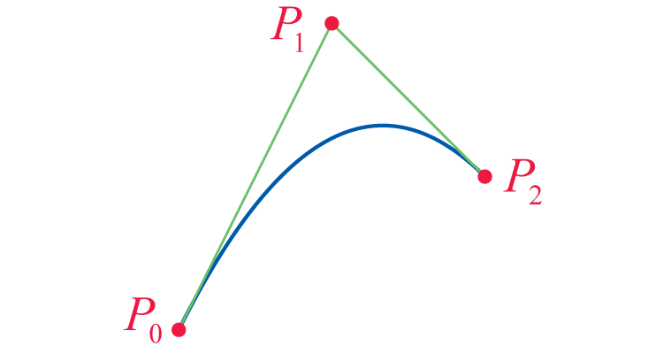
   Three points labeled P₀, P₁, and P₂, moving from left to right and connected in sequence. P0 lies below the other two points, P1 lies above the other two points. A quadratic curve opening downward connects P0 and P2.

3. The cubic Bézier curve $B_{0,1,2,3}\left(t\right)$ with control points $P_0$, $P_1$, $P_2$, and $P_3$ joins $P_0$ and $P_3$ so that the line segments $\overline{P_0{P}_1}$ and $\overline{P_2{P}_3}$ are tangent to $B_{0,1,2,3}\left(t\right)$ at $P_0$ and $P_3$, respectively (see Figure 2). Verify that the following curve satisfies these conditions.

   $x\left(t\right)=a_0{\left(1-t\right)}^3+3a_1{\left(1-t\right)}^{2}t+3a_2\left(1-t\right)t^2+a_3{t}^3$

   $\phantom{t\in \left[0,1\right]}y\left(t\right)=b_0{\left(1-t\right)}^3+3b_1{\left(1-t\right)}^{2}t+3b_2\left(1-t\right)t^2+b_3{t}^3$, $t\in \left[0,1\right]$

   

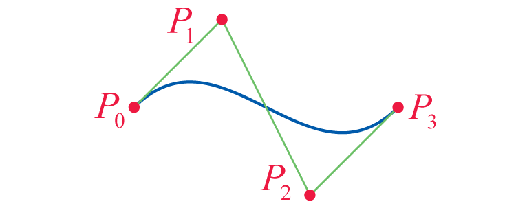
   Four points labeled P₀, P₁, P₂, and P₃, moving from left to right and connected in sequence. P1 lies above the other three points, P2 lies below the other three points. P₀ and P₁ are at the same height. A cubic curve connects P₀ and P₃, curving upwards towards P₂ and curving downwards towards P₃.

4. Show that the parametrization in Question 3 corresponds to

   $B_{0,1,2,3}\left(t\right)=\left(1-t\right)B_{0,1,2}\left(t\right)+t{B}_{1,2,3}\left(t\right)$.

5. Use Question 3 to verify that the Bézier curve with control points $P_0\left(1,3\right)$, $P_1\left(3,7\right)$, $P_2\left(6,9\right)$, and $P_3\left(8,6\right)$ has the following parametrization

   $x\left(t\right)=-2t^3+3t^2+6t+1$

   $y\left(t\right)=-3t^3-6t^2+12t+3$

6. Find the slope of the curve in Question 5 at

   1. $t=0$,

   2. $t={\displaystyle \frac{1}{2}}$,

   3. $t=1$

7. Use a computer algebra system to graph the Bézier curve of Question 5 along with its control points. If your CAS has animation capabilities, explore what happens if you move around the control points in the plane.